FOURIER TRANSFORM
| Fourier transforms |
|---|
| Continuous Fourier transform |
| Fourier series |
| Discrete-time Fourier transform |
| Discrete Fourier transform |
|
|
|
|
The Fourier transform, named for Joseph Fourier, is a mathematical transform with many applications in physics and engineering. Very commonly, it expresses a mathematical function of time as a function of frequency, known as its frequency spectrum. The Fourier inversion theorem details this relationship. For instance, the transform of a musical chord made up of pure notes (without overtones) expressed as amplitude as a function of time, is a mathematical representation of the amplitudes and phases of the individual notes that make it up. The function of time is often called the time domain representation, and the frequency spectrum the frequency domain representation. The inverse Fourier transform expresses a frequency domain function in the time domain. Each value of the function is usually expressed as a complex number (called complex amplitude) that can be interpreted as a magnitude and a phase component. The term "Fourier transform" refers to both the transform operation and to the complex-valued function it produces.
In the case of a periodic function, such as a continuous, but not necessarily sinusoidal, musical tone, the Fourier transform can be simplified to the calculation of a discrete set of complex amplitudes, called Fourier series coefficients. Also, when a time-domain function is sampled to facilitate storage or computer-processing, it is still possible to recreate a version of the original Fourier transform according to the Poisson summation formula, also known as discrete-time Fourier transform. These topics are addressed in separate articles. For an overview of those and other related operations, refer to Fourier analysis or List of Fourier-related transforms.
Definition
There are several common conventions for defining the Fourier transform ƒ̂ of an integrable function ƒ: R → C (Kaiser 1994, p. 29), (Rahman 2011, p. 11). This article will use the definition:
-
 , for every real number ξ.
When the independent variable x represents time (with SI unit of seconds), the transform variable ξ represents frequency (in hertz). Under suitable conditions, ƒ can be reconstructed from ƒ̂ by the inverse transform:
-
 for every real number x.
The statement that ƒ can be reconstructed from ƒ̂ is known as the Fourier integral theorem, and was first introduced in Fourier's Analytical Theory of Heat (Fourier 1822, p. 525), (Fourier & Freeman 1878, p. 408), although what would be considered a proof by modern standards was not given until much later (Titchmarsh 1948, p. 1). The functions ƒ and ƒ̂ often are referred to as a Fourier integral pair or Fourier transform pair (Rahman 2011, p. 10).
For other common conventions and notations, including using the angular frequency ω instead of the frequency ξ, see Other conventions and Other notations below. The Fourier transform on Euclidean space is treated separately, in which the variable x often represents position and ξ momentum.
Example
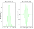
The following images provide a visual illustration of how the Fourier transform measures whether a frequency is present in a particular function. The function depicted ƒ(t) = cos(6πt) e-πt2 oscillates at 3 hertz (if t measures seconds) and tends quickly to 0. (The second factor in this equation is an envelope function that shapes the continuous sinusoid into a short pulse. Its general form is a Gaussian function). This function was specially chosen to have a real Fourier transform which can easily be plotted. The first image contains its graph. In order to calculate ƒ̂(3) we must integrate e−2πi(3t)ƒ(t). The second image shows the plot of the real and imaginary parts of this function. The real part of the integrand is almost always positive, because when ƒ(t) is negative, the real part of e−2πi(3t) is negative as well. Because they oscillate at the same rate, when ƒ(t) is positive, so is the real part of e−2πi(3t). The result is that when you integrate the real part of the integrand you get a relatively large number (in this case 0.5). On the other hand, when you try to measure a frequency that is not present, as in the case when we look at ƒ̂(5), the integrand oscillates enough so that the integral is very small. The general situation may be a bit more complicated than this, but this in spirit is how the Fourier transform measures how much of an individual frequency is present in a function ƒ(t).
-

Original function showing oscillation 3 hertz.
-
Real and imaginary parts of integrand for Fourier transform at 3 hertz
-

Real and imaginary parts of integrand for Fourier transform at 5 hertz
-

Fourier transform with 3 and 5 hertz labeled.


